Simple Linear Regression in Machine Learning (ML)

In machine learning, linear regression is a commonly used technique for modeling the relationship between a dependent variable and one or more independent variables, also known as features or predictors.

Why Linear Regression?

Linear regression in machine learning is a popular and widely used technique because it is relatively simple and interpretable, and it can often achieve good performance on a wide range of problems. Also whatever we learn in linear regression, we can implement in other machine learning algorithms.

Linear regression is a supervised learning algorithm, which means that it requires labeled data to train the model. There are several types of linear regression that can be used depending on the specific problem and data at hand. Some of the most common types of linear regression include:

1. Simple linear regression: This is the most basic type of linear regression, where there is only one independent variable and one dependent variable. The goal is to find a linear relationship between the two variables.
2. Multiple linear regression: This type of linear regression involves more than one independent variable, and the goal is to find a linear relationship between the independent variables and the dependent variable.
3. Polynomial regression: This type of linear regression is used when the relationship between the independent variable and the dependent variable is not linear but can be approximated by a polynomial function.

Let’s Understand the Simple Linear Regression in depth.

Simple Linear Regression

Simple linear regression is a statistical method used to model the relationship between two variables by fitting a linear equation to the data. One variable (usually denoted as “x”) is considered as the predictor or independent variable, while the other variable (usually denoted as “y”) is the response or dependent variable.

The equation for simple linear regression is:

y = β0 + β1*x + ε

Where,
y — dependent variable
x — independent variable
β0 — intercept
β1 — coefficient of x
ε — error term

In simple linear regression, we try to find the best-fit line that explains the relationship between x and y. This line is called the regression line.

Code Example

Here’s an example of simple linear regression in Python:

import numpy as np
import pandas as pd
import matplotlib.pyplot as plt
from sklearn.linear_model import LinearRegression

# generate some random data for x and y
x = np.array([1, 2, 3, 4, 5])
y = np.array([2, 4, 5, 6, 7])

# visualize the data using scatter plot
plt.scatter(x, y)
plt.xlabel('x')
plt.ylabel('y')
plt.show()

# create a linear regression model and fit the data
model = LinearRegression()
model.fit(x.reshape(-1, 1), y)

# predict the values of y using the model
y_pred = model.predict(x.reshape(-1, 1))

# visualize the regression line
plt.scatter(x, y)
plt.plot(x, y_pred, color='red')
plt.xlabel('x')
plt.ylabel('y')
plt.show()

# print the coefficients of the linear regression model
print('Intercept:', model.intercept_)
print('Coefficient:', model.coef_)

In this example, we generated some random data for x and y and visualized the data using a scatter plot. We then created a linear regression model using the LinearRegression class from scikit-learn, and fitted the data to the model. We then used the model to predict the values of y for the given values of x. Finally, we visualized the regression line and printed the coefficients of the linear regression model.

The output of this code will be:

Intercept: 1.5
Coefficient: [1.1]

This means that the intercept of the regression line is 1.5, and the coefficient of x is 1.1. Therefore, the equation of the regression line is:

y = 1.5 + 1.1*x

This equation can be used to predict the value of y for any given value of x.

Intuition

In the example code I provided, we were trying to model the relationship between x and y, where x was the independent variable and y was the dependent variable. The scatter plot of the data showed that there was a positive correlation between x and y, which means that as x increases, y also increases.

The linear regression model we created used the data to find the best-fit line that could explain this relationship. The line was found by minimizing the sum of the squared distances between the actual data points and the predicted values on the line. This line can then be used to predict the values of y for any given value of x.

In the output of the code, we can see that the intercept of the line is 1.5 and the coefficient of x is 1.1. This means that if x=0, then y=1.5, and for every unit increase in x, y increases by 1.1.

Overall, simple linear regression is a valuable tool for understanding the relationship between two variables and can be used to make predictions about the dependent variable based on the independent variable.

How to find m(slop) and b(intercept)

The formula for the slope (m) and intercept (b) in simple linear regression can be derived as follows:

Let (x1, y1), (x2, y2), …, (xn, yn) be the n data points. We want to find the values of m and b that minimize the sum of the squared differences between the actual y values and the predicted y values on the line. This can be written as:

min Σ(yi — (mx + b))²

To find the values of m and b that minimize this expression, we can take partial derivatives with respect to m and b and set them equal to zero.

Taking the partial derivative with respect to m, we get:

∂/∂m Σ(yi — (mx + b))² = -2Σxi(yi — (mx + b))

Setting this equal to 0 and solving for m, we get:

Σxiyi — nxb = mΣxi²

Dividing both sides by Σxi², we get:

m = (Σxiyi — nxb) / Σxi²

Taking the partial derivative with respect to b, we get:

∂/∂b Σ(yi — (mx + b))² = -2Σ(yi — (mx + b))

Setting this equal to 0 and solving for b, we get:

Σyi — mΣxi = nb

Dividing both sides by n, we get:

b = ȳ — mx̄

where ȳ and x̄ are the means of the y and x values, respectively. This gives us the formula for the slope (m) and intercept (b) in terms of the sample means and sums of products and squares. Once we have calculated m and b using these formulas, we can use them to create the regression equation:

y = mx + b

This equation represents the line of best fit that describes the relationship between x and y in the data.

Code from Scratch for Simple Linear Regression

Here’s an example implementation of simple linear regression in Python using the least squares method:

import numpy as np

class SimpleLinearRegression:
    
    def __init__(self):
        self.slope = None
        self.intercept = None
        
    def fit(self, X, y):
        n = len(X)
        x_mean = np.mean(X)
        y_mean = np.mean(y)
        
        # Calculate the sums of squares and products
        ss_xy = np.sum(X*y) - n*x_mean*y_mean
        ss_xx = np.sum(X*X) - n*x_mean*x_mean
        
        # Calculate the slope and intercept
        self.slope = ss_xy / ss_xx
        self.intercept = y_mean - self.slope*x_mean
        
    def predict(self, X):
        return self.slope*X + self.intercept

Here’s an explanation of the code:

1. We import the NumPy library for numerical calculations.
2. We define a SimpleLinearRegression class that contains methods for fitting the model and making predictions.
3. In the constructor (__init__), we initialize the slope and intercept attributes to None.
4. The fit method takes in the predictor variable X and the target variable y as input. It calculates the sample means of X and y, and then uses them to calculate the slope and intercept of the regression line using the formulas derived earlier. These values are stored in the slope and intercept attributes of the object.
5. The predict method takes in a new set of X values and returns the corresponding predicted y values using the fitted regression line.

To use this implementation, you would create an instance of the SimpleLinearRegression class, call the fit method with your training data, and then call the predict method with new test data to obtain predictions. Here's an example usage:

# Create a simple linear regression object
regressor = SimpleLinearRegression()

# Generate some random data
X = np.array([1, 2, 3, 4, 5])
y = np.array([2, 4, 5, 4, 6])

# Fit the regression line to the data
regressor.fit(X, y)

# Make predictions for new data
X_new = np.array([6, 7, 8])
y_pred = regressor.predict(X_new)

# Print the predicted values
print(y_pred)

Output : [6.4 7.8 9.2]

Regression Metrics | MSE, MAE & RMSE | R2 Score & Adjusted R2 Score

Regression metrics are quantitative measures that evaluate the performance of regression models. Regression metrics help to assess how well a regression model is able to predict the output variable.

MAE (Mean Absolute Error)

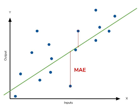
The MAE is the average absolute difference between the predicted and actual values. It measures the average magnitude of the errors in the predictions. The formula for Mean Absolute Error (MAE) is:

MAE = (1/n) * Σ|i=1 to n| |yᵢ — ȳ|

where:

n is the total number of observations
yᵢ is the predicted value for the i-th observation
ȳ is the actual value for the i-th observation

The MAE is expressed in the same units as the output variable, making it easy to interpret the magnitude of the errors. It is less sensitive to outliers compared to other regression metrics like MSE and RMSE. However, It does not take into account the direction of the errors, meaning overpredictions and underpredictions are treated equally. It gives equal weight to all errors, regardless of their magnitude or importance.

MSE (Mean Squared Error)

Mean Squared Error (MSE) is a regression metric that is used to evaluate the performance of a regression model. It solves the problem of assessing how well a regression model is able to fit the data and make accurate predictions.

The main problem that MSE solves is to quantify the average squared difference between the predicted and actual values of the output variable. This metric penalizes larger errors more heavily than smaller errors, as it squares each difference before averaging. By squaring the errors, the metric emphasizes the importance of larger errors that may have a greater impact on the model’s overall performance.

In summary, MSE and MAE solve different problems in regression modeling. MSE emphasizes the importance of larger errors and is more sensitive to outliers, while MAE treats all errors equally and is less sensitive to outliers. The choice between these metrics depends on the specific requirements of the problem and the nature of the data.

Root Mean Squared Error (RMSE)

RMSE is the square root of the Mean Squared Error (MSE), which is another common regression metric.

The need for RMSE arises from the fact that MSE has a squared unit, which can make it difficult to interpret and compare across different datasets. By taking the square root of MSE, RMSE expresses the errors in the same units as the output variable, making it easier to interpret the magnitude of the errors. RMSE is widely used in machine learning and statistics as a measure of model performance, particularly in cases where the output variable has a natural scale or units of measurement.

Squared R (R²)

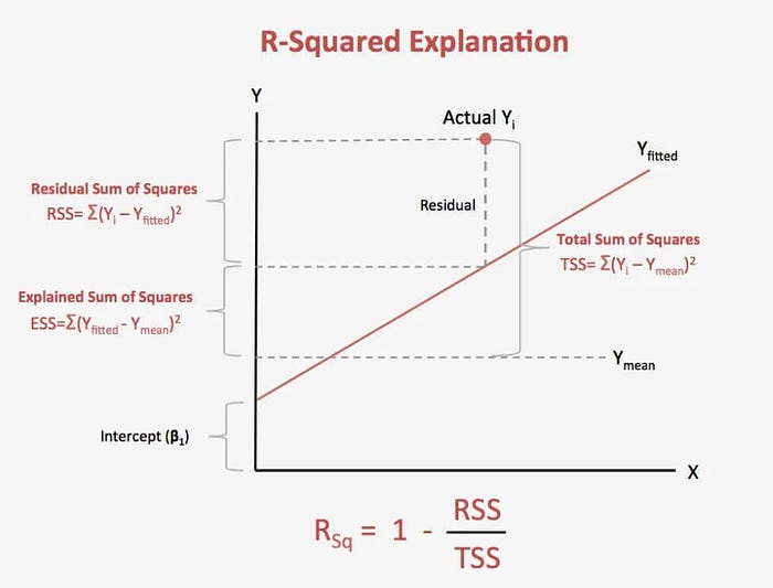
Squared R (R²) is a regression metric that measures the proportion of variance in the dependent variable that can be explained by the independent variable(s) in a regression model. R² is a statistical measure that ranges from 0 to 1, with higher values indicating a better fit between the model and the data.

The need for R² arises from the fact that regression models are used to predict the values of a dependent variable based on one or more independent variables. The goal of regression modeling is to build a model that can accurately predict the values of the dependent variable based on the independent variables. R² provides a measure of how well the model fits the data and how much of the variability in the dependent variable can be explained by the independent variable(s).

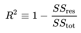
The formula for R² is:

where:

• SSres is the sum of the squared residuals or errors (the difference between the predicted and actual values) from the regression model
• SStot is the total sum of squares or the sum of the squared differences between the actual values and the mean of the dependent variable

A value of R² = 0 indicates that the regression model does not explain any of the variances in the dependent variable, while a value of R² = 1 indicates that the regression model perfectly explains all of the variances in the dependent variable. However, in practice, it is rare for a regression model to have an R² value of exactly 1.

Adjusted R-squared

Adjusted R-squared is a variant of R-squared that adjusts for the number of independent variables in a regression model. While R-squared provides a measure of the goodness-of-fit of a regression model, Adjusted R-squared takes into account the number of independent variables in the model and provides a more conservative estimate of the proportion of variance in the dependent variable that is explained by the independent variable(s).

The formula for Adjusted R-squared is:

Adjusted R² = 1 — [(1 — R²) * (n — 1) / (n — k — 1)]

where:

• R² is the R-squared value
• n is the number of observations in the data set
• k is the number of independent variables in the model

Adjusted R-squared is used to compare the performance of regression models with different numbers of independent variables. It penalizes the addition of unnecessary independent variables to the model, which can lead to overfitting and reduced generalization performance. Adjusted R-squared will always be lower than R-squared when additional independent variables are added to the model.

A higher Adjusted R-squared value indicates a better fit between the regression model and the data, while a lower Adjusted R-squared value indicates a worse fit. However, like R-squared, Adjusted R-squared should be used in conjunction with other regression metrics and visualizations to fully evaluate the performance of a regression model.

Check the code below link:

100-days-of-machine-learning/day49-regression-metrics at main ·…